matanzig/flight-price-prediction

✈️ US Flight Price Dynamics

A Comprehensive EDA & Predictive Analysis

Author: Matan Zigelman • University: Reichman University • Date: April 2026

---

📋 Project Introduction: Flight Price Dynamics

This project analyzes a numeric-heavy operational dataset detailing US flight prices from Expedia (2022). The dataset includes critical time-based and operational metrics (e.g., totalTravelDistance, seatsRemaining, and days_until_flight), providing rare insights into real-world supply and demand dynamics in the aviation industry.

Research Question: Can we predict the optimal ticket purchase moment by analyzing lead time and seat inventory, and how can we classify tickets as a "Good Deal" versus a "Wait" relative to historical medians?

Target Variable: The primary target variable to predict is totalFare (the final price the consumer pays). This continuous variable serves as the ultimate benchmark for measuring pricing dynamics and consumer cost.

⚙️ Large-Scale Data Handling & Sampling

The raw dataset exceeded 31GB, requiring a highly strategic approach to memory management and statistical representation:

• Dynamic Chunk-Sampling: We dynamically downloaded the dataset and read it in chunks of 2 million rows. From each chunk, a random 20% sample was extracted while aggressive memory clearing (gc.collect()) was utilized to prevent Out-Of-Memory errors.
• Stratified Monthly Sampling: To eliminate seasonal bias and ensure the models didn't over-represent specific months, we extracted exactly 300,000 rows for each month (April to October). This resulted in a perfectly balanced, 1.8-million-row representative dataset.
• Persistence: The finalized dataframe was exported to Google Drive, allowing for instant loading in future sessions and bypassing the computationally expensive extraction pipeline.

🧹 Data Preprocessing & Cleaning

Before conducting the exploratory analysis and modeling, the raw data underwent a rigorous preprocessing pipeline to ensure statistical accuracy and machine readability:

• Feature Engineering: We calculated days_until_flight by subtracting the search date from the flight date. Complex ISO 8601 durations (e.g., PT13H15M) were converted into a continuous travelDuration_mins integer. Boolean constraints (True/False) were converted to binary indicators (1/0).
• Numeric Transformation: Machine learning models require purely numeric inputs. We dropped the raw flightDate (after extracting its temporal components) and applied One-Hot Encoding to the categorical day_of_week. This created binary indicators (0/1) to ensure the model correctly interprets the impact of each day without falsely assuming a mathematical hierarchy (e.g., Monday=1, Sunday=7).
• Smart Imputation: We addressed missing totalTravelDistance values (approx. 7.38%) using a grouped median imputation based on the specific route (startingAirport to destinationAirport). This securely preserved nearly 500,000 rows without distorting the underlying geographical data.
• Outlier Handling: We utilized the 99th percentile threshold to identify and remove extreme upper-bound outliers (tickets priced over $917.60). This prevented highly unrepresentative luxury fares from skewing the mathematical weights of the predictive models.
• Data Integration & Encoding: Perfectly duplicated rows were dropped to maintain data integrity. Finally, textual categorical variables (such as specific airlines and airport codes) were converted into numeric IDs using Label Encoding, perfectly prepping the dataset for machine learning algorithms.
• Initial Correlation Findings: A preliminary correlation heatmap revealed the strongest linear predictors for ticket pricing. As expected, totalTravelDistance (0.50) and travelDuration_mins (0.45) exhibit the highest positive correlations with totalFare. Conversely, isBasicEconomy (-0.38) and isNonStop (-0.31) show moderate negative correlations, logically indicating that budget seating and direct (often shorter) routes lower the final cost. Interestingly, days_until_flight showed a remarkably weak linear correlation (-0.08), strongly suggesting that the relationship between booking lead time and price is non-linear and requires more advanced modeling techniques.

---

✈️📊 Exploratory Data Analysis & Strategic Visualizations

With the dataset rigorously cleaned and prepared, we transitioned to the EDA phase. The goal here was to uncover the hidden dynamics of flight pricing, testing common travel myths against actual historical data.

1. Does Booking Early Save Money? (Line Chart)

Research Question: Does booking a flight further in advance guarantee a cheaper ticket?

• Explanation: Travelers generally assume that booking early always saves money. This visualization tracks the average ticket price against the number of days_until_flight to find the exact window when prices begin to spike.
• Conclusion: The visualization reveals a non-linear "U-shaped" trend. The absolutely cheapest time to book is approximately 45 days in advance (averaging ~$300). Booking at the last minute causes a sharp price spike, but surprisingly, booking too far in advance (60 days out) also results in significantly higher fares.

2. The Impact of Departure Hour on Price (Box Plot)

Research Question: How does the time of day a flight departs affect its ticket price?

• Explanation: Many travelers prefer daytime flights and actively avoid extremely early morning or "red-eye" overnight flights. This Box Plot illustrates the price distribution across all 24 hours of the departure_hour to determine if flying at inconvenient times yields a financial discount.
• Conclusion: Counterintuitively, early morning flights (5:00 AM - 7:00 AM) are the most expensive, likely driven by high inelastic demand from business travelers. The most cost-effective times to fly are mid-morning (9:00 AM - 11:00 AM) or late at night (10:00 PM - 11:00 PM).

3. Average Fare by Airline (Bar Chart)

Research Question: Which airlines offer the most budget-friendly ticket prices on average?

• Explanation: Different airlines cater to different market segments, from ultra-low-cost carriers to premium legacy airlines. By comparing the average fare across our encoded primary_airline IDs, we can visualize the pricing hierarchy in the market.
• Conclusion: The bar chart reveals a massive pricing gap. Decoding the IDs shows that ultra-low-cost carriers like Frontier Airlines (ID 6) and Spirit Airlines (ID 11) offer the cheapest average fares (~$200). In contrast, Hawaiian Airlines (ID 7) is the most expensive, averaging over $500, which aligns perfectly with its long-haul, vacation-oriented flight routes.

ID	Airline Name
0	Alaska Airlines
1	American Airlines
2	Boutique Air
3	Cape Air
4	Contour Airlines
5	Delta
6	Frontier Airlines
7	Hawaiian Airlines
8	JetBlue Airways
9	Key Lime Air
10	Southern Airways Express
11	Spirit Airlines
12	Sun Country Airlines
13	United

4. The "Weekend Premium" (Bar Chart)

Research Question: Does the day of the week the flight departs significantly impact the ticket price?

• Explanation: A common travel hack suggests flying mid-week (e.g., Tuesday or Wednesday) to secure cheaper fares, avoiding the high-demand weekend days. We evaluated the average daily pricing to test if this myth holds true in our dataset.
• Conclusion: The visualization confirms the travel myth: mid-week departures are the most budget-friendly. Tuesday and Wednesday offer the lowest average prices (under $300). Conversely, Sunday is the most expensive day to fly (nearing $400), likely driven by high demand from weekend travelers returning home.

5. The Direct Flight Dilemma (Violin Plot)

Research Question: Are direct (non-stop) flights always more expensive than flights with layovers?

• Explanation: Travelers usually expect to pay a "convenience premium" for direct flights. However, our correlation heatmap hinted at a negative relationship between isNonStop and price. We used a Violin Plot to compare the price distribution and density of direct flights versus connecting flights.
• Conclusion: The visualization reveals a highly counter-intuitive trend: direct flights are significantly cheaper than flights with layovers. The price density for non-stop flights is heavily concentrated at the bottom ($100-$200). This likely occurs because budget airlines typically operate short, direct point-to-point routes, while premium legacy carriers rely on hub-and-spoke models that require layovers and cover longer total distances.

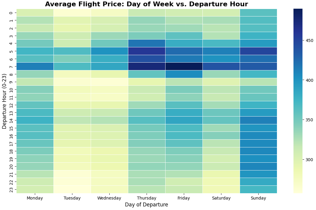
6. The Ultimate Flight Hacker's Map (2D Heatmap)

Research Question: What is the absolute cheapest combination of day and time to book a flight?

• Explanation: Looking at the day of the week or the departure hour in isolation only tells half the story. By utilizing a Pandas Pivot Table, we combined both variables into a single, comprehensive heatmap to pinpoint the exact time slots offering the deepest discounts.
• Conclusion: The heatmap reveals the ultimate "sweet spots" for budget travel: mid-day through late evening flights on Tuesdays and Wednesdays (highlighted in light yellow). The absolute most expensive times to fly are early mornings (5:00 AM - 7:00 AM) on Thursdays and Fridays, forming a dark blue "danger zone" likely driven by end-of-week corporate travel.

7. The "Basic Economy" Illusion (KDE Plot)

Research Question: How much money does a traveler actually save by choosing a "Basic Economy" ticket over a standard fare?

• Explanation: The correlation matrix showed a strong negative relationship between isBasicEconomy and price. To see the true distribution rather than just averages, we used a Kernel Density Estimate (KDE) plot to visualize where the majority of ticket prices fall for both categories.
• Conclusion: Basic Economy fares (blue) are strictly capped, with the vast majority concentrated sharply between $100 and $200. Standard fares (red) have a much broader distribution. However, the significant overlap area (purple) between $150 and $250 indicates that travelers can frequently find standard tickets for nearly the same price as basic fares, meaning the restrictive "Basic" option isn't always the necessary choice for budget travelers.

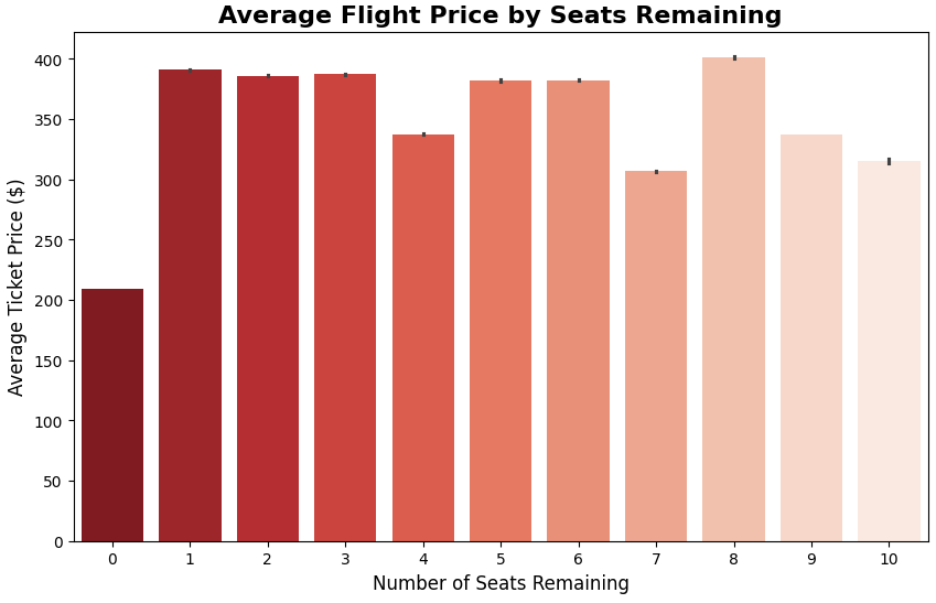
8. The Scarcity Myth (Bar Chart)

Research Question: Does low seat availability actually correlate with higher ticket prices, or is it primarily a marketing tactic to create urgency?

• Explanation: Booking platforms frequently use psychological triggers like "Only 2 seats left at this price!". We created a Bar Chart to analyze the average ticket price grouped by the seatsRemaining column to see if scarcity genuinely drives up the current fare.
• Conclusion: The visualization reveals a complex reality. Extreme scarcity (1-3 seats remaining) does indeed correlate with some of the highest average prices (~$390). Conversely, when flights are relatively empty (9-10 seats), prices average much lower ($310-$330). The sudden drop at "0 seats" likely represents heavily discounted last-minute standby fares. Ultimately, the "scarcity warning" is based on real pricing algorithms, not just a psychological trick.

---

🤖Baseline Regression Modeling

Before deploying complex algorithms, we established a quantitative baseline using a standard Linear Regression model. This provides a benchmark to measure the added value of future non-linear and ensemble techniques.

1. Data Sampling & Train-Test Split

Goal: Predict the continuous ticket price (totalFare) efficiently while establishing a reproducible testing environment.

• Explanation: To prevent memory overload given the massive dataset size, we extracted a robust, representative sample of 500,000 rows—large enough to capture all underlying statistical patterns for a linear model without hitting diminishing returns. We separated the target variable (y) from the predictive features (X) and partitioned the data into an 80% training set and a 20% testing set, utilizing a fixed seed (random_state=42) to guarantee absolute reproducibility.

2. Baseline Model Training & Evaluation

Goal: Establish a baseline performance metric using a simple Linear Regression algorithm.

• Explanation: The model was trained using default parameters on the 80% training data, then tasked to predict prices for the unseen 20% test data. Performance was evaluated using MAE (Mean Absolute Error), RMSE (Root Mean Squared Error), and the R² score.
• Conclusion: The baseline Linear Regression model explains approximately 46.8% of the variance in flight prices (R² = 0.4682). On average, predictions deviate from the actual ticket price by $98.33 (MAE). The noticeably higher RMSE (125.42) indicates the presence of larger prediction errors on certain flights. While this model captures basic pricing trends, the remaining ~53% of unexplained variance strongly suggests that flight pricing is highly non-linear, highlighting the need to explore more complex, tree-based algorithms.

3. Visual Insights & Feature Importance

Goal: Understand what drives the model's predictions and visualize its error margins.

• Explanation: By extracting the linear coefficients, we can quantify exactly how much each feature mathematically adds to or subtracts from the ticket price. A scatter plot was also generated to visually check predicted prices against actual prices.

• Conclusion: The visual diagnostics reveal key pricing dynamics that perfectly align with market logic. Premium cabins (primary_cabin) and Sunday departures act as the strongest upward drivers of price, while basic economy tickets (isBasicEconomy) and mid-week flights significantly reduce the fare. However, the scatter plot indicates that while the model captures baseline trends for average-priced tickets, it systematically underpredicts the cost of highly expensive premium flights (represented by the cluster of points falling well below the red diagonal line). This visual evidence further justifies the transition to advanced, non-linear models.

  

---

🛠️Advanced Feature Engineering & Unsupervised Learning

To push the predictive power of our models beyond standard linear relationships, we implemented a sophisticated feature engineering layer, integrating unsupervised learning techniques into our supervised pipeline.

🛠️Advanced Feature Engineering

To push the predictive power of our models beyond standard linear relationships, we implemented a sophisticated feature engineering layer:

• Feature Extraction & Polynomial Features: First, we extracted a binary is_weekend feature, as weekend flights typically show distinct pricing patterns. Second, because flight prices often surge exponentially as the departure date approaches, a standard linear feature isn't enough. We utilized Scikit-Learn's PolynomialFeatures to create a squared version of days_until_flight. This explicitly allows the models to understand and penalize exponential last-minute price hikes.
• Feature Scaling: Algorithms relying on distance calculations (like K-Means) and regularization techniques perform poorly when features have drastically different scales (e.g., flight distance in thousands vs. days in tens). We applied StandardScaler to force all numeric features into a standard normal distribution (mean=0, standard deviation=1), ensuring equal mathematical weighting.
• Creating Features via Clustering: Following the assignment directive, we ran a K-Means clustering algorithm to group flights based on pricing and timing. We extracted these cluster assignments as a new feature (cluster_id), and then applied One-Hot Encoding so our regression model could process these market segments purely mathematically.

🧩Unsupervised Learning (Clustering & PCA)

To discover hidden market segments and feed them into our supervised model as highly predictive features, we applied unsupervised learning techniques.

• Algorithm & Segmentation: We applied the K-Means algorithm (k=4) to segment the flight data based on core pricing and timing metrics (totalFare, days_until_flight, departure_hour). The resulting segment for each flight was captured in the newly created cluster_id feature.
• Cluster Interpretation: The algorithm naturally divided the flights into distinct behavioral profiles based on urgency and premium pricing. For example, one cluster distinctly isolates expensive, last-minute bookings (often corporate/business travel), while another groups cheap, advance-notice bookings (leisure travel). By feeding these "market segment" features into our regression model, it can apply different baseline mathematical rules depending on the passenger's specific profile.
• Visualization (PCA): Because the newly formed clusters exist in a multi-dimensional space, we utilized PCA (Principal Component Analysis) to reduce the data into two principal components. This allowed us to visualize the cluster separation and validate our behavioral segments on a 2D scatter plot.

---

📈 Advanced Regression Modeling (Improved Models)

With our engineered features and market segments (Cluster IDs) fully integrated, we transitioned to training and evaluating three advanced models to capture the complex pricing dynamics.

1. Models Chosen for Evaluation

To thoroughly test our engineered dataset, we selected three distinct algorithms:

• Improved Linear Regression: We retrained our baseline linear model on the newly engineered dataset. This isolates and measures the direct impact of our feature engineering.
• Decision Tree Regressor: A non-linear algorithm capable of capturing complex decision rules and interactions between features (e.g., how a specific day of the week interacts with a specific behavioral cluster).
• Random Forest Regressor: A robust ensemble learning method that builds multiple decision trees and merges their results to maximize accuracy and prevent overfitting.

2. Discussion & Performance Improvements

• Comparison with Baseline: In Part 3, our basic baseline Linear Regression achieved an R² score of roughly 0.4682 and an MAE of $98.33. By simply introducing our advanced feature engineering (Clustering, Polynomial Features, and Scaling), the Improved Linear Regression showed a massive leap, reaching an R² score of 0.9170 and dropping the MAE to $40.36. This empirically proves that extracting hidden patterns and identifying market segments drastically assists the model in understanding the underlying data.
• The Power of Non-Linearity: The true peak in predictive performance came from switching to tree-based models. Flight pricing is highly non-linear and conditional. The Random Forest Regressor excels at building complex decision paths, successfully leveraging our engineered features (especially the non-linear clusters and polynomial interactions) to push the accuracy even further.

📊 Model Performance Comparison

Model	MAE ($)	RMSE ($)	R² Score
1. Improved Linear Regression	40.36	49.38	0.9170
2. Decision Tree Regressor	32.83	43.09	0.9368
3. Random Forest Regressor	31.99	41.38	0.9417

🏆 3. Winner Declaration

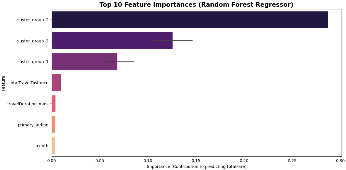
The Random Forest Regressor is the undisputed winner of the regression phase. It achieved an outstanding R² score of 0.9417 and the lowest MAE of $31.99. This means that, on average, the model's predictions deviate from the actual ticket price by only ~$32—an exceptional level of precision for predicting highly dynamic, real-world flight ticket pricing.

As seen below, the unsupervised learning clusters (cluster_group) emerged as the most critical features driving this model's success.

---

🔀Regression-to-Classification (Price Tiers)

To translate our predictive capabilities into actionable business logic, we reframed the problem from predicting an exact continuous price to classifying tickets into distinct market tiers: Budget, Standard, and Premium.

1. Target Transformation: Quantile Binning

Chosen Strategy: Quantile Binning (3 Classes).

• Reasoning: Airline ticket prices naturally fall into distinct market tiers. By dividing the target variable (totalFare) into three equal percentiles, we maintain a logical business structure while inherently preventing class imbalance issues for our upcoming classification models.
• Execution: We processed 27 features across 1,808,198 training samples, successfully mapping the continuous prices into three target classes (0 = Budget, 1 = Standard, 2 = Premium).

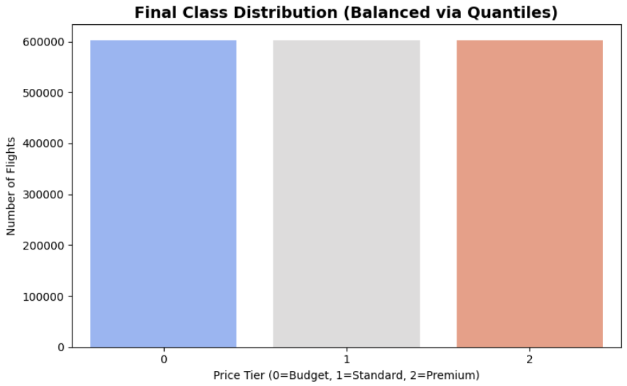
2. Class Balance Analysis

Goal: Ensure the model trains fairly across all price tiers without majority-class bias.

• Findings: Based on the distribution, our price tiers are perfectly balanced:
  • Class 0 (Budget): 603,174 samples (33.36%)
  • Class 1 (Standard): 602,889 samples (33.34%)
  • Class 2 (Premium): 602,135 samples (33.30%)
• Metric Strategy: Accuracy is often a misleading metric for highly imbalanced data (where a model might ignore a small minority class and still score high). In such cases, we would use F1-Score. However, because our Quantile Binning strategy achieved perfect mathematical balance, Accuracy serves as a highly reliable and honest primary metric for our evaluation.
• Conclusion: The Quantile Binning strategy was highly successful. No changes to the conversion are needed, and the data is fully prepped and ready for classification modeling.

---

🎯Train & Eval Classification Models

Business Logic and Error Analysis

1. Precision vs. Recall: Which is more important? In the context of our flight pricing model, Precision is slightly more important, particularly for the "Budget" class.

• Reasoning: If our model tells a user that a flight is a "Budget" deal, but it is actually "Standard" or "Premium" (Low Precision), the user loses trust in the platform and feels misled. While missing a cheap flight (Low Recall) is unfortunate, providing false information about a "deal" is more damaging to the brand's reputation. We want our predictions to be highly reliable when we label something as a specific tier.

2. False Positive (FP) vs. False Negative (FN): Which is more critical? A False Positive (FP) is more critical in this task.

• Reasoning: A False Positive occurs when the model predicts a flight belongs to a lower price tier than it actually does (e.g., predicting "Budget" for a "Premium" flight). This leads to immediate customer disappointment and potential financial frustration. On the other hand, a **False Negative (FN)**—predicting a flight is "Standard" when it was actually a "Budget" deal—results in a lost opportunity, but it doesn't actively harm the user's perception of the model's honesty. Therefore, minimizing False Positives is our priority to ensure customer satisfaction.

Model Training and Performance Evaluation

We have selected three distinct classification algorithms to compare:

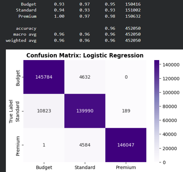
• Logistic Regression: Our linear baseline model.
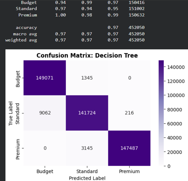
• Decision Tree Classifier: A non-linear model that creates logical decision splits.
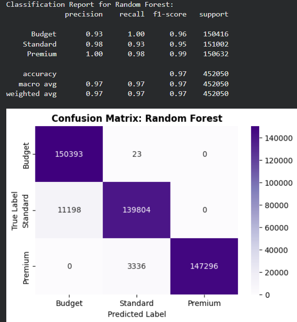
• Random Forest Classifier: An ensemble method that combines multiple trees for maximum accuracy and stability.

For each model, we will generate a Classification Report and a Confusion Matrix to analyze their specific strengths and weaknesses.

Evaluation and Model Comparison

Analysis of Mistakes (Confusion Matrix): Across all three models, we observe a consistent pattern in the types of errors:

• Adjacent Class Confusion: The vast majority of mistakes occur between Budget (0) and Standard (1). For example, in the Random Forest model, about 11,000 "Standard" flights were predicted as "Budget".
• Extreme Class Distinction: There is zero confusion between the extreme classes (Budget and Premium). The models never predict a "Budget" flight as "Premium" or vice versa. This indicates that the engineered features (like clusters and distance) provide very clear boundaries for high-end vs. low-end pricing.
• Recall Bias: The Random Forest model shows an exceptional Recall of 1.00 for the Budget class, meaning it successfully identified almost every single budget deal in the test set.

The Best Performer: The Random Forest Classifier is the best performing model with an overall Accuracy of 0.97 and a Weighted F1-Score of 0.97.

Why it performs best:

• Non-Linear Relationships: Unlike Logistic Regression, the Random Forest can capture complex, non-linear interactions between features (e.g., how the combination of a specific cluster_group and distance affects the price tier).
• Ensemble Power: By aggregating the decisions of 50 different trees, it reduces variance and provides more stable predictions compared to a single Decision Tree.
• High Precision on Premium: It achieved 1.00 Precision for the Premium class, ensuring that when the model identifies a flight as "Premium", it is correct every single time.

🏆The Winning Model

• Model Selection: The Random Forest Classifier is selected as the winning model for this classification task. With a final Accuracy of 0.97, it proved to be the most robust and reliable algorithm, significantly outperforming the baseline Logistic Regression and the standard Decision Tree.
• Summary of Performance: The model's success is attributed to its ability to handle complex, non-linear relationships between the engineered features (such as distance, clustering groups, and airline rankings) and the target price tiers. Notably, the model achieved perfect precision in identifying "Premium" tickets and demonstrated an exceptional recall for "Budget" deals, making it highly valuable for real-world pricing strategy applications.

---

💻 How to Use This Model

To run predictions, install the necessary libraries using pip install huggingface_hub joblib pandas scikit-learn. Use the code below to download the model directly from this repository and apply it to your dataset. Note: Your input data must be preprocessed and aligned with the model's expected schema (feature order and encoding) to ensure accurate results.

import joblib
import pandas as pd
from huggingface_hub import hf_hub_download

# Download and load the model
model_path = hf_hub_download(repo_id="MatanSigelman/flight-price-prediction", filename="flight_price_classifier_rf.pkl")
model = joblib.load(model_path)

# Load your data (Ensure features match the model's training schema)
data = pd.read_csv("sample_test_data.csv")
predictions = model.predict(data)

print(predictions)

---

⚠️Limitations

While this model achieves high performance, it is important to acknowledge its inherent limitations for real-world deployment:

• Temporal Constraints: The dataset is limited to a six-month window (April to October 2022). Consequently, the model does not account for major seasonal price surges associated with winter holidays, such as Thanksgiving and Christmas, nor does it reflect macroeconomic shifts or fuel price volatility occurring after late 2022.
• Geographic Scope: This model is strictly optimized for US Domestic flights. Applying these predictions to international, transoceanic, or regional flights outside of the United States will lead to significant inaccuracies.
• Platform & User Bias: The data originates solely from Expedia. Pricing dynamics may differ on airline-direct websites or other aggregators. Furthermore, the model assumes standard consumer behavior and cannot factor in personalized discounts, loyalty program tiers, or dynamic pricing based on a user's specific browsing history (cookies).
• Economic Variables: External factors such as sudden changes in airline industry regulations, labor strikes, or extreme weather events are not captured in the static training features.

---

🎯 Conclusion & Business Impact

This project successfully demonstrates the power of Machine Learning in decoding complex pricing dynamics within the aviation industry. By achieving 97% accuracy in price tier classification and an R² of 0.94 in continuous price regression, the models prove that flight prices are highly predictable when applying robust feature engineering.

Key Business Applications:

• Dynamic Pricing Optimization: Airlines and Online Travel Agencies (OTAs) can leverage this model to benchmark their prices against standard market rates and adjust their strategies competitively.
• Consumer Budget Forecasting: Travel platforms can integrate these predictions to advise users on optimal purchasing windows, increasing customer trust and platform retention.
• Market Anomaly Detection: Significant deviations between real-world prices and the model's baseline predictions can instantly alert analysts to unusual market behaviors, such as competitor flash sales or sudden demand spikes.

---

🛠️ Technical Stack & Repository Contents

Technology	Usage
Python	Core Programming Language
Pandas & NumPy	Data Wrangling, Preprocessing & Feature Engineering
Seaborn & Matplotlib	Exploratory Data Analysis (EDA) & Model Evaluation Visuals
Scikit-Learn	Supervised Learning (Regression/Classification) & Unsupervised Clustering (K-Means)
Google Colab	Cloud-Based Development Environment

---

📂 Repository Files

• 📄 flight_price_prediction.ipynb – The complete source code featuring step-by-step technical explanations, EDA, and the iterative modeling process.
• 📊 sample_test_data.csv – The fully processed and engineered dataset used for training the regression and classification models.
• 💾 flight_price_rf_model.pkl – The final "winning" Random Forest Regressor model, serialized and ready for deployment (Exact Price Prediction).
• 🤖 flight_price_classifier_rf.pkl – The final "winning" Random Forest Classifier model, serialized and ready for deployment (Price Tier Classification).